


CDA数据分析师 出品
作者:CDA教研组
编辑:Mika
案例介绍
背景:以某大型电商平台的用户行为数据为数据集,使用大数据处理技术分析海量数据下的用户行为特征,并通过建立逻辑回归模型、随机森林对用户行为做出预测;
案例思路:
- 使用大数据处理技术读取海量数据
- 海量数据预处理
- 抽取部分数据调试模型
- 使用海量数据搭建模型
#全部行输出
from IPython.core.interactiveshell import InteractiveShell
InteractiveShell.ast_node_interactivity = “all”
数据字典:
U_Id:the serialized ID that represents a user
T_Id:the serialized ID that represents an item
C_Id:the serialized ID that represents the category which the corresponding item belongs to Ts:the timestamp of the behavior
Be_type:enum-type from (‘pv’, ‘buy’, ‘cart’, ‘fav’)
pv: Page view of an item’s detail page, equivalent to an item click
buy: Purchase an item
cart: Add an item to shopping cart
fav: Favor an item
读取数据
这里关键是使用dask库来处理海量数据,它的大多数操作的运行速度比常规pandas等库快十倍左右。
pandas在分析结构化数据方面非常的流行和强大,但是它最大的限制就在于设计时没有考虑到可伸缩性。pandas特别适合处理小型结构化数据,并且经过高度优化,可以对存储在内存中的数据执行快速高 效的操作。然而随着数据量的大幅度增加,单机肯定会读取不下的,通过集群的方式来处理是最好的选 择。这就是Dask DataFrame API发挥作用的地方:通过为pandas提供一个包装器,可以智能的将巨大的DataFrame分隔成更小的片段,并将它们分散到多个worker(帧)中,并存储在磁盘中而不是RAM中。
Dask DataFrame会被分割成多个部门,每个部分称之为一个分区,每个分区都是一个相对较小的 DataFrame,可以分配给任意的worker,并在需要复制时维护其完整数据。具体操作就是对每个分区并 行或单独操作(多个机器的话也可以并行),然后再将结果合并,其实从直观上也能推出Dask肯定是这么做的。
# 安装库(清华镜像)
# pip install dask -i https://pypi.tuna.tsinghua.edu.cn/simple
import os
import gc # 垃圾回收接口
from tqdm import tqdm # 进度条库
import dask # 并行计算接口
from dask.diagnostics import ProgressBar
import numpy as np
import pandas as pd
import matplotlib.pyplot as plt
import time
import dask.dataframe as dd # dask中的数表处理库 import sys # 外部参数获取接口
面对海量数据,跑完一个模块的代码就可以加一行gc.collect()来做内存碎片回收,Dask Dataframes与Pandas Dataframes具有相同的API
gc.collect()
42
# 加载数据
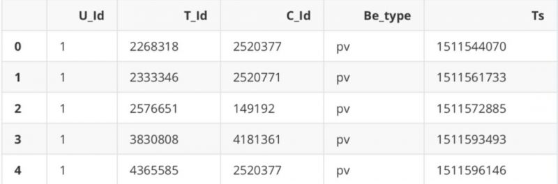
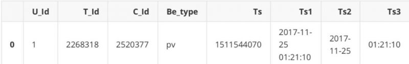
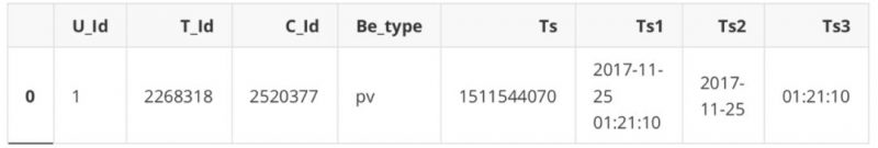
data = dd.read_csv(‘UserBehavior_all.csv’)# 需要时可以设置blocksize=参数来手工指定划分方法,默认是64MB(需要设置为总线的倍数,否则会放慢速度)
data.head()
.dataframe tbody tr th {
vertical-align: top;
}
.dataframe thead th {
text-align: right;
}
data
Dask DataFrame Structure :
.dataframe tbody tr th {
vertical-align: top;
}
.dataframe thead th {
text-align: right;
}
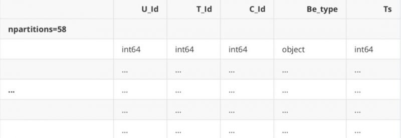
Dask Name: read-csv, 58 tasks
与pandas不同,这里我们仅获取数据框的结构,而不是实际数据框。Dask已将数据帧分为几块加载,这些块存在 于磁盘上,而不存在于RAM中。如果必须输出数据帧,则首先需要将所有数据帧都放入RAM,将它们缝合在一 起,然后展示最终的数据帧。使用.compute()强迫它这样做,否则它不.compute() 。其实dask使用了一种延迟数 据加载机制,这种延迟机制类似于python的迭代器组件,只有当需要使用数据的时候才会去真正加载数据。
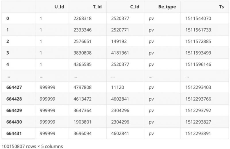
# 真正加载数据 data.compute()
.dataframe tbody tr th {
vertical-align: top;
}
.dataframe thead th {
text-align: right;
}
# 可视化工作进程,58个分区任务 data.visualize()
数据预处理
数据压缩
# 查看现在的数据类型 data.dtypes
U_Id int64
T_Id int64
C_Id int64
Be_type object
Ts int64
dtype: object
# 压缩成32位uint,无符号整型,因为交易数据没有负数 dtypes = {
‘U_Id’: ‘uint32’,
‘T_Id’: ‘uint32’,
‘C_Id’: ‘uint32’,
‘Be_type’: ‘object’,
‘Ts’: ‘int64’
}
data = data.astype(dtypes)
data.dtypes
U_Id uint32
T_Id uint32
C_Id uint32
Be_type object
Ts int64
dtype: object
缺失值
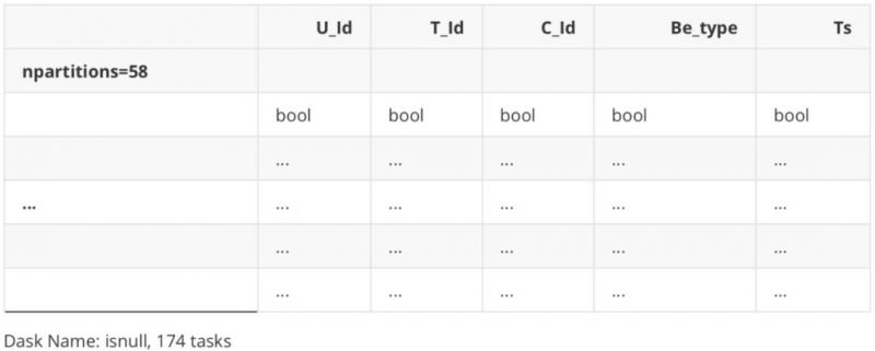
# 以dask接口读取的数据,无法直接用.isnull()等pandas常用函数筛查缺失值
data.isnull()
Dask DataFrame Structure :
.dataframe tbody tr th {
vertical-align: top;
}
.dataframe thead th {
text-align: right;
}
columns1 = [ ‘U_Id’, ‘T_Id’, ‘C_Id’, ‘Be_type’, ‘Ts’]
tmpDf1 = pd.DataFrame(columns=columns1)
tmpDf1
.dataframe tbody tr th {
vertical-align: top;
}
.dataframe thead th {
text-align: right;
}

s = data[“U_Id”].isna()
s.loc[s == True]
Dask Series Structure:
npartitions=58
bool …
… …
…
Name: U_Id, dtype: bool
Dask Name: loc-series, 348 tasks
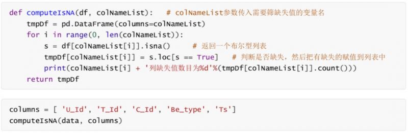
U_Id列缺失值数目为0
T_Id列缺失值数目为0
C_Id列缺失值数目为0
Be_type列缺失值数目为0
Ts列缺失值数目为0
.dataframe tbody tr th {
vertical-align: top;
}
.dataframe thead th {
text-align: right;
}

无缺失值
数据探索与可视化
这里我们使用pyecharts库。pyecharts是一款将python与百度开源的echarts结合的数据可视化工具。新版的1.X和旧版的0.5.X版本代码规则大 不相同,新版详见官方文档https://gallery.pyecharts.org/#/README
# pip install pyecharts -i https://pypi.tuna.tsinghua.edu.cn/simple
Looking in indexes: https://pypi.tuna.tsinghua.edu.cn/simple
Requirement already satisfied: pyecharts in d:\anaconda\lib\site-packages (0.1.9.4)
Requirement already satisfied: jinja2 in d:\anaconda\lib\site-packages (from pyecharts)
(3.0.2)
Requirement already satisfied: future in d:\anaconda\lib\site-packages (from pyecharts)
(0.18.2)
Requirement already satisfied: pillow in d:\anaconda\lib\site-packages (from pyecharts)
(8.3.2)
Requirement already satisfied: MarkupSafe>=2.0 in d:\anaconda\lib\site-packages (from
jinja2->pyecharts) (2.0.1)
Note: you may need to restart the kernel to use updated packages.
U_Id列缺失值数目为0 T_Id列缺失值数目为0 C_Id列缺失值数目为0 Be_type列缺失值数目为0 Ts列缺失值数目为0
WARNING: Ignoring invalid distribution -umpy (d:\anaconda\lib\site-packages)
WARNING: Ignoring invalid distribution -ip (d:\anaconda\lib\site-packages)
WARNING: Ignoring invalid distribution -umpy (d:\anaconda\lib\site-packages)
WARNING: Ignoring invalid distribution -ip (d:\anaconda\lib\site-packages)
WARNING: Ignoring invalid distribution -umpy (d:\anaconda\lib\site-packages)
WARNING: Ignoring invalid distribution -ip (d:\anaconda\lib\site-packages)
WARNING: Ignoring invalid distribution -umpy (d:\anaconda\lib\site-packages)
WARNING: Ignoring invalid distribution -ip (d:\anaconda\lib\site-packages)
WARNING: Ignoring invalid distribution -umpy (d:\anaconda\lib\site-packages)
WARNING: Ignoring invalid distribution -ip (d:\anaconda\lib\site-packages)
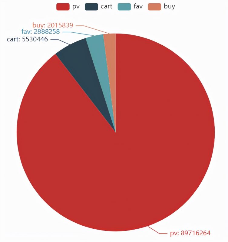
饼图
# 例如,我们想画一张漂亮的饼图来看各种用户行为的占比 data[“Be_type”]
# 使用dask的时候,所有支持的原pandas的函数后面需加.compute()才能最终执行
Be_counts = data[“Be_type”].value_counts().compute()
Be_counts
pv 89716264
cart 5530446
fav 2888258
buy 2015839
Name: Be_type, dtype: int64
Be_index = Be_counts.index.tolist() # 提取标签
Be_index
[‘pv’, ‘cart’, ‘fav’, ‘buy’]
Be_values = Be_counts.values.tolist() # 提取数值
Be_values
[89716264, 5530446, 2888258, 2015839]
from pyecharts import options as opts
from pyecharts.charts import Pie
#pie这个包里的数据必须传入由元组组成的列表
c = Pie()
c.add(“”, [list(z) for z in zip(Be_index, Be_values)]) # zip函数的作用是将可迭代对象打包成一 个个元组,然后返回这些元组组成的列表 c.set_global_opts(title_opts=opts.TitleOpts(title=”用户行为”)) # 全局参数(图命名) c.set_series_opts(label_opts=opts.LabelOpts(formatter=”{b}: {c}”))
c.render_notebook() # 输出到当前notebook环境
# c.render(“pie_base.html”) # 若需要可以将图输出到本机
<pyecharts.charts.basic_charts.pie.Pie at 0x1b2da75ae48>
<div id=”490361952ca944fcab93351482e4b254″ style=”width:900px; height:500px;”></div>
漏斗图
from pyecharts.charts import Funnel # 旧版的pyecharts不需要.charts即可import import pyecharts.options as opts
from IPython.display import Image as IMG
from pyecharts import options as opts
from pyecharts.charts import Pie

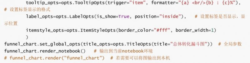
<pyecharts.charts.basic_charts.funnel.Funnel at 0x1b2939d50c8>
<div id=”071b3b906c27405aaf6bc7a686e36aaa” style=”width:800px; height:400px;”></div>

数据分析
时间戳转换
dask对于时间戳的支持非常不友好
type(data)
dask.dataframe.core.DataFrame
data[‘Ts1’]=data[‘Ts’].apply(lambda x: time.strftime(“%Y-%m-%d %H:%M:%S”,
time.localtime(x)))
data[‘Ts2’]=data[‘Ts’].apply(lambda x: time.strftime(“%Y-%m-%d”, time.localtime(x)))
data[‘Ts3’]=data[‘Ts’].apply(lambda x: time.strftime(“%H:%M:%S”, time.localtime(x)))
D:\anaconda\lib\site-packages\dask\dataframe\core.py:3701: UserWarning:
You did not provide metadata, so Dask is running your function on a small dataset to
guess output types. It is possible that Dask will guess incorrectly.
To provide an explicit output types or to silence this message, please provide the
`meta=` keyword, as described in the map or apply function that you are using.
Before: .apply(func)
After: .apply(func, meta=(‘Ts’, ‘object’))
warnings.warn(meta_warning(meta))
data.head(1)
.dataframe tbody tr th {
vertical-align: top;
}
.dataframe thead th {
text-align: right;
}
data.dtypes
U_Id uint32
T_Id uint32
C_Id uint32
Be_type object
Ts int64
Ts1 object
Ts2 object
Ts3 object
dtype: object
抽取一部分数据来调试代码
df = data.head(1000000)
df.head(1)
.dataframe tbody tr th {
vertical-align: top;
}
.dataframe thead th {
text-align: right;
}
用户流量和购买时间情况分析
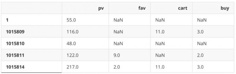
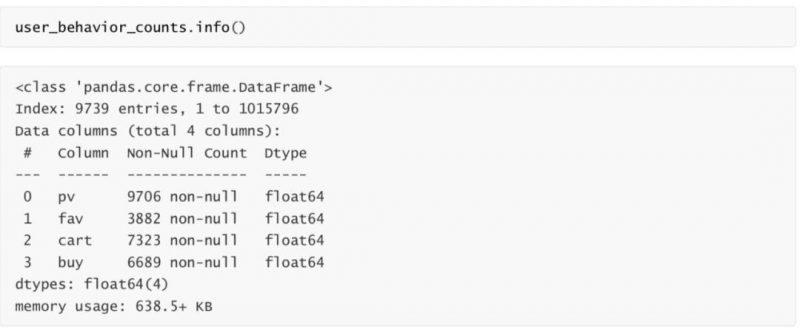
用户行为统计表
describe = df.loc[:,[“U_Id”,”Be_type”]]
ids = pd.DataFrame(np.zeros(len(set(list(df[“U_Id”])))),index=set(list(df[“U_Id”])))
pv_class=describe[describe[“Be_type”]==”pv”].groupby(“U_Id”).count()
pv_class.columns = [“pv”]
buy_class=describe[describe[“Be_type”]==”buy”].groupby(“U_Id”).count()
buy_class.columns = [“buy”]
fav_class=describe[describe[“Be_type”]==”fav”].groupby(“U_Id”).count()
fav_class.columns = [“fav”]
cart_class=describe[describe[“Be_type”]==”cart”].groupby(“U_Id”).count()
cart_class.columns = [“cart”]
user_behavior_counts=ids.join(pv_class).join(fav_class).join(cart_class).join(buy_class).
iloc[:,1:]
user_behavior_counts.head()
.dataframe tbody tr th {
vertical-align: top;
}
.dataframe thead th {
text-align: right;
}
总访问量成交量时间变化分析(天)
from matplotlib import font_manager
# 解决坐标轴刻度负号乱码
# 解决负号’-‘显示为方块的问题 plt.rcParams[‘axes.unicode_minus’] = False # 解决中文乱码问题 plt.rcParams[‘font.sans-serif’] = [‘Simhei’]
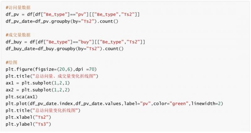

由总访问量、成交量时间变化分析知,从17年11月25日至17年12月1日访问量和成交量存在小幅波动,2017年12 月2日访问量和成交量均出现大幅上升,2日、3日两天保持高访问量和高成交量。此现象原因之一为12月2日和3 日为周末,同时考虑2日3日可能存在某些促销活动,可结合实际业务情况进行具体分析。(图中周五访问量有上 升,但成交量出现下降,推测此现象可能与周末活动导致周五推迟成交有关。)
总访问量成交量时间变化分析(小时)
# 数据准备 df_pv_timestamp=df[df[“Be_type”]==”pv”][[“Be_type”,”Ts1″]] df_pv_timestamp[“Ts1”] = pd.to_datetime(df_pv_timestamp[“Ts1”])
df_pv_timestamp=df_pv_timestamp.set_index(“Ts1”)
df_pv_timestamp=df_pv_timestamp.resample(“H”).count()[“Be_type”]
df_pv_timestamp
df_buy_timestamp=df[df[“Be_type”]==”buy”][[“Be_type”,”Ts1″]]
df_buy_timestamp[“Ts1”] = pd.to_datetime(df_buy_timestamp[“Ts1”])
df_buy_timestamp=df_buy_timestamp.set_index(“Ts1”)
df_buy_timestamp=df_buy_timestamp.resample(“H”).count()[“Be_type”]
df_buy_timestamp
Ts1
2017-09-11 16:00:00 1
2017-09-11 17:00:00 0
2017-09-11 18:00:00 0
2017-09-11 19:00:00 0
2017-09-11 20:00:00 0
…
2017-12-03 20:00:00 8587
2017-12-03 21:00:00 10413
2017-12-03 22:00:00 9862
2017-12-03 23:00:00 7226
2017-12-04 00:00:00 1
Freq: H, Name: Be_type, Length: 2001, dtype: int64
Ts1
2017-11-25 00:00:00 64
2017-11-25 01:00:00 29
2017-11-25 02:00:00 18
2017-11-25 03:00:00 8
2017-11-25 04:00:00 3
…
2017-12-03 19:00:00 141
2017-12-03 20:00:00 159
2017-12-03 21:00:00 154
2017-12-03 22:00:00 154
2017-12-03 23:00:00 123
Freq: H, Name: Be_type, Length: 216, dtype: int64
#绘图
plt.figure(figsize=(20,6),dpi =70)
x2= df_buy_timestamp.index plt.plot(range(len(x2)),df_buy_timestamp.values,label=”成交量”,color=”blue”,linewidth=2) plt.title(“总成交量变化折现图(小时)”)
x2 = [i.strftime(“%Y-%m-%d %H:%M”) for i in x2]
plt.xticks(range(len(x2))[::4],x2[::4],rotation=90)
plt.xlabel(“Ts2”)
plt.ylabel(“Ts3”)
plt.grid(alpha=0.4);

特征工程
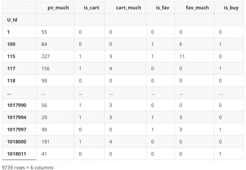
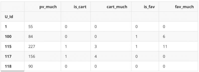
思路:不考虑时间窗口,只以用户的点击和收藏等行为来预测是否购买 流程:以用户ID(U_Id)为分组键,将每位用户的点击、收藏、加购物车的行为统计出来,分别为
是否点击,点击次数;是否收藏,收藏次数;是否加购物车,加购物车次数
以此来预测最终是否购买
# 去掉时间戳
df = df[[“U_Id”, “T_Id”, “C_Id”, “Be_type”]] df
.dataframe tbody tr th {
vertical-align: top;
}
.dataframe thead th {
text-align: right;
}
行为类型
U_Id
1 [1,1,1,1,1,1,1,1,1,1,1,1,1,1,1,…
100 [1,1,1,1,1,1,1,1,1,3,1,1,3,1,3,…
115 [1,1,1,1,1,1,1,1,1,1,1,1,1,1,3,…
117 [4,1,1,1,1,1,1,4,1,1,1,1,1,1,1,…
118 [1,1,1,1,1,1,1,1,1,1,1,1,1,1,1,…
Name: Be_type1, dtype: object
最后创建一个DataFrame用来存储等下计算出的用户行为。
df_new = pd.DataFrame()
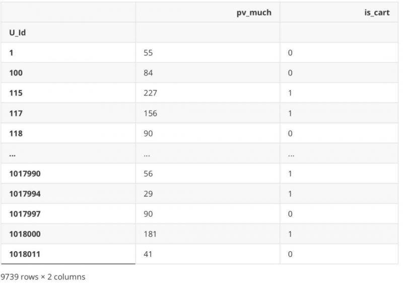
点击次数
df_new[‘pv_much’] = df_Be.apply(lambda x: Counter(x)[‘1’])
df_new
.dataframe tbody tr th {
vertical-align: top;
}
.dataframe thead th {
text-align: right;
}
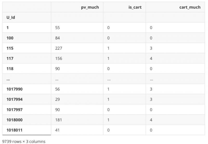
加购次数
#是否加购
df_new[‘is_cart’] = df_Be.apply(lambda x: 1 if ‘2’ in x else 0)
df_new
.dataframe tbody tr th {
vertical-align: top;
}
.dataframe thead th {
text-align: right;
}
#加购了几次
df_new[‘cart_much’] = df_Be.apply(lambda x: 0 if ‘2’ not in x else Counter(x)[‘2’])
df_new
.dataframe tbody tr th {
vertical-align: top;
}
.dataframe thead th {
text-align: right;
}
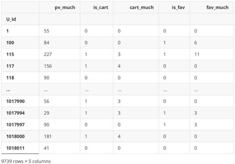
收藏次数
#是否收藏
df_new[‘is_fav’] = df_Be.apply(lambda x: 1 if ‘3’ in x else 0)
df_new
.dataframe tbody tr th {
vertical-align: top;
}
.dataframe thead th {
text-align: right;
}

#收藏了几次
df_new[‘fav_much’] = df_Be.apply(lambda x: 0 if ‘3’ not in x else Counter(x)[‘3’])
df_new
.dataframe tbody tr th {
vertical-align: top;
}
.dataframe thead th {
text-align: right;
}
相关分析
#部分数据 df_new.corr(‘spearman’)
.dataframe tbody tr th {
vertical-align: top;
}
.dataframe thead th {
text-align: right;
}
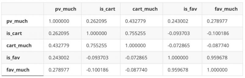
是否加购与加购次数、是否收藏与收藏次数之间存在一定相关性,但经验证剔除其中之一与纳入全部变量效果基本一致,故之后使用全部变量建模。
数据标签
import seaborn as sns
#是否购买
df_new[‘is_buy’] = df_Be.apply(lambda x: 1 if ‘4’ in x else 0)
df_new
.dataframe tbody tr th {
vertical-align: top;
}
.dataframe thead th {
text-align: right;
}
df_new.is_buy.value_counts()
1 6689
0 3050
Name: is_buy, dtype: int64
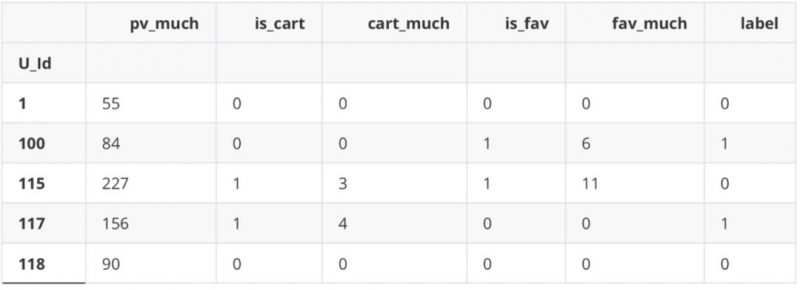
df_new[‘label’] = df_new[‘is_buy’]
del df_new[‘is_buy’]
df_new.head()
.dataframe tbody tr th {
vertical-align: top;
}
.dataframe thead th {
text-align: right;
}
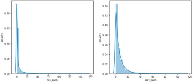
f,ax=plt.subplots(1,2,figsize=(12,5))
sns.set_palette([“#9b59b6″,”#3498db”,]) #设置所有图的颜色,使用hls色彩空间
sns.distplot(df_new[‘fav_much’],bins=30,kde=True,label=’123′,ax=ax[0]);
sns.distplot(df_new[‘cart_much’],bins=30,kde=True,label=’12’,ax=ax[1]);
C:\Users\CDA\anaconda3\lib\site-packages\seaborn\distributions.py:2619: FutureWarning:
`distplot` is a deprecated function and will be removed in a future version. Please adapt
your code to use either `displot` (a figure-level function with similar flexibility) or
`histplot` (an axes-level function for histograms).
warnings.warn(msg, FutureWarning)
建立模型
划分数据集
from sklearn.model_selection import train_test_split
X = df_new.iloc[:,:-1]
Y = df_new.iloc[:,-1]
X.head()
Y.head()
.dataframe tbody tr th {
vertical-align: top;
}
.dataframe thead th {
text-align: right;
}
U_Id
10
100 1
115 0
117 1
118 0
Name: label, dtype: int64
Xtrain,Xtest,Ytrain,Ytest = train_test_split(X,Y,test_size= 0.3,random_state= 42)
逻辑回归
模型建立
from sklearn.linear_model import LogisticRegression
LR_1 = LogisticRegression().fit(Xtrain,Ytrain)
#简单测试 LR_1.score(Xtest,Ytest)
0.6741957563312799
模型评估
from sklearn import metrics
from sklearn.metrics import classification_report
from sklearn.metrics import auc,roc_curve
#混淆矩阵
print(metrics.confusion_matrix(Ytest, LR_1.predict(Xtest)))
[[ 0 952]
[ 0 1970]]
print(classification_report(Ytest,LR_1.predict(Xtest)))
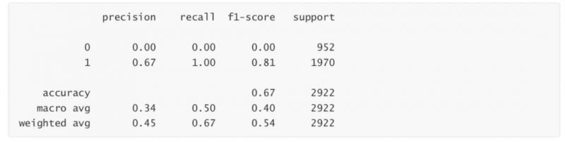
D:\anaconda\lib\site-packages\sklearn\metrics\_classification.py:1308:
UndefinedMetricWarning: Precision and F-score are ill-defined and being set to 0.0 in
labels with no predicted samples. Use `zero_division` parameter to control this behavior.
_warn_prf(average, modifier, msg_start, len(result))
D:\anaconda\lib\site-packages\sklearn\metrics\_classification.py:1308:
UndefinedMetricWarning: Precision and F-score are ill-defined and being set to 0.0 in
labels with no predicted samples. Use `zero_division` parameter to control this behavior.
_warn_prf(average, modifier, msg_start, len(result))
D:\anaconda\lib\site-packages\sklearn\metrics\_classification.py:1308:
UndefinedMetricWarning: Precision and F-score are ill-defined and being set to 0.0 in
labels with no predicted samples. Use `zero_division` parameter to control this behavior.
_warn_prf(average, modifier, msg_start, len(result))
fpr,tpr,threshold = roc_curve(Ytest,LR_1.predict_proba(Xtest)[:,1])
roc_auc = auc(fpr,tpr)
print(roc_auc)
0.6379193682549162
随机森林
模型建立
from sklearn.ensemble import RandomForestClassifier
rfc = RandomForestClassifier(n_estimators=200, max_depth=1)
rfc.fit(Xtrain, Ytrain)
RandomForestClassifier(max_depth=1, n_estimators=200)
模型评估
#混淆矩阵
print(metrics.confusion_matrix(Ytest, rfc.predict(Xtest)))
[[ 0 952]
[ 0 1970]]
#分类报告
print(metrics.classification_report(Ytest, rfc.predict(Xtest)))
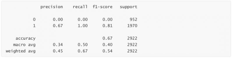
D:\anaconda\lib\site-packages\sklearn\metrics\_classification.py:1308:
UndefinedMetricWarning: Precision and F-score are ill-defined and being set to 0.0 in
labels with no predicted samples. Use `zero_division` parameter to control this behavior.
_warn_prf(average, modifier, msg_start, len(result))
D:\anaconda\lib\site-packages\sklearn\metrics\_classification.py:1308:
UndefinedMetricWarning: Precision and F-score are ill-defined and being set to 0.0 in
labels with no predicted samples. Use `zero_division` parameter to control this behavior.
_warn_prf(average, modifier, msg_start, len(result))
D:\anaconda\lib\site-packages\sklearn\metrics\_classification.py:1308:
UndefinedMetricWarning: Precision and F-score are ill-defined and being set to 0.0 in
labels with no predicted samples. Use `zero_division` parameter to control this behavior.
_warn_prf(average, modifier, msg_start, len(result))
原创文章,作者:运营增长,如若转载,请注明出处:https://ziliaobaba.com/10136.html